Random processes/ Noise generators

The purpose is to generate a "noisy" value centered on zero ( ie with Mean= 0), which is more or less related to the previous step output value ( ie more or less correlated ), and to allow to set the standard deviation of the output when a statistically stationary state is reached. Added to an ideal value, this can simulate errors/perturbations.

The equations of numerical generators are general. Their parameters are further defined so that they are also a simulation of their continuous counterpart, in order to make them independent of the Timestep( delay between to updates); the code is written that way.

By definition, the covariance is the square of the standard deviation, ie Cov= StdDev². For random processes as defined below, the covariance of the ouput can be computed: it is worth noticing that its equations are deterministic and can be computed separately from the perturbation equation.
This allow for a selection of an appropriate perturbation generator based on its statistical properties which are deterministic, where the standard deviation can be viewed as a measurement of the generated output inaccuracy.

"w01" denotes gaussian white noise, with mean= 0 and standard deviation= 1, as provided by the function RVgauss01() below.
"w0S" denotes gaussian white noise, with mean= 0 and standard deviation= StdDev_w0S, which can be modelled as wOS= StdDev_w0S* w01.

1^st order noise generator

The following implementation is based on a first order low-pass filter input by a gaussian white noise.
X_n= K *X_n-1+ W0S or X_n= K *X_n-1+ StdDev_WOS* W01, with 0 < K < 1
X₀=X(n=0), StdDev_x₀ and StdDev_WOS are given.
The covariance Cov_X of the output is given by
Cov_X_n= K²* Cov_X_n-1+ Cov_WOS.
For constant Cov_WOS and K, this can be solved as:
Cov_X_n= Cov_X₀*K²ⁿ+ (1- K²ⁿ)*Cov_WOS /(1- K²) Note that Cov_X varies like the output of a first order filter running twice faster than the X filter, with initial condition Cov_X₀ and input being a step= Cov_WOS/(1-K²).
Correlation ( smoothing) increases with K increasing from 0 to 1.
Calls to the float RVgauss01() function will return values for W01.

The statistically stationary state is reached when n tends towards infinity, where our requirement is StdDev_x_SteadyState= StdDevOut, assuming a constant Cov_WOS.
As Cov_X_SteadyState= K_StdDevOut² by definition,
and Cov_X_SteadyState= Cov_WOS/(1-K²), we must set StdDev_WOS= K_StdDevOut* sqrt(1- K²).
The corresponding continuous noise generator is
dx/dt= -k*x+ b*w01, hence
dCov_x/dt= -2 *k *Cov_x+ b².
To simulate it, we must set K= exp(-k T) and K_StdDevOut= b/sqrt(2k), T being the timestep.

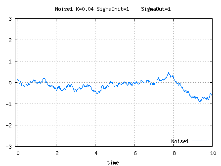
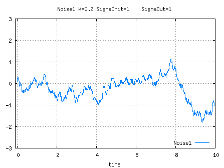
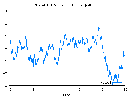
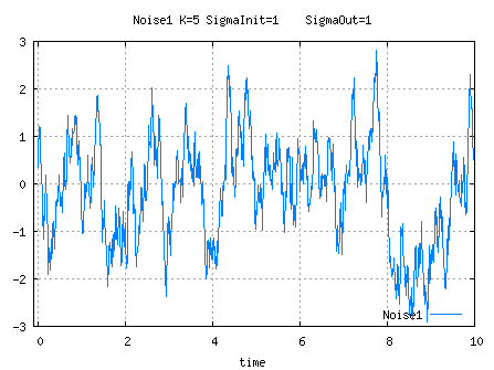
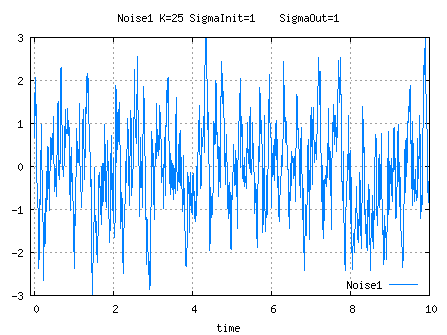
NF1Noise
float g_output, StdDev_WOS, StdDevInit;
//at init time
void initcoloredNoise1()
{
//_ compute K= exp(-k*T)...see first order linear filter

StdDev_WOS= K_StdDevOut* sqrt(1- K*K);

//_ to get constant statistical characteristics right from the start
StdDevInit= K_StdDevOut;
//_
g_output= StdDevInit*RVgauss01();
}
//------------
float coloredNoise1()
{
return g_output= K* g_output+ StdDev_WOS* RVgauss01();
}

Using Filter N1LL ( where A= 1-K) with input= StdDev_w0S/A*W01 is another equivalent implementation.

Random walk

For high values of K, the output as defined hereabove slowly drifts but its covariance is bounded , which somehow bounds the drift. To get an unbounded drift, one should use a "random walk", ie
X_n= X_n-1+ T* StdDev_WOS* W01.
X₀ and StdDev_X₀ are given.
The output covariance is:
Cov_X_n= Cov_X_n-1+ T²* Cov_WOS.
For a constant Cov_WOS, this can be solved as: Cov_X_n= Cov_X₀+ n* T²* Cov_WOS.

The continuous formulation is:
dx/dt= b* wo1, hence
dCov_x/dt= b².
Cov_WOS must then be equal to b²/T, and Cov_X varies then linearly with time as:
Cov_X_n= Cov_X₀+ n* T* b².

2^nd order noise generator

This generator provides more short-term "damping" than the 1st order one.
StdDevOut is the desired standard deviation of the output. The equations shows 2 variables, and the covariance is now a 2x2 positive semi_definite matrix CovMat.In particular, CovMat= CovMat^T, ie CovMat does not change by exchanging rows and column: CovMat12= CovMat21.
X_n= -K₁* X_n-1 -K₀* Y_n-1+ A * StdDev_WOS *W01, with A= 1+K₀+K₁
Y_n= X_n-1
X₀, Y₀, CovMat₀ are given. To have a nice transient curve for covariances, I strongly suggest , once CovMat11₀= CovMat12₀ has been set, to set CovMat12₀=CovMat21₀=-K₁* CovMat11₀/(1+K₀) and initialize Y₀ from X₀ as done in the code.
The general formula to get CovMat variations can be simplified (!) as:
CovMat11_n= K₁²*CovMat11_n-1+ 2* K₁*K₀*CovMat12_n-1 + K₁²*CovMat22_n-1+ A² * Cov_WOS
CovMat12_n= -K₁*CovMat11_n-1- K₀*CovMat12_n-1
CovMat22_n=CovMat11_n-1.
In statistical steady state:
Cov_X=CovMat11= CovMat22= Cov_WOS* A*(1+GA0)/((1-K₀)(1+K₀-K₁)) and
Cov_XY= CovMat12= CovMat22= -K₁* CovMat11/(1+K₀).

Examples with Damping Coeff= 1.0

Examples with Damping Coeff= 0.3

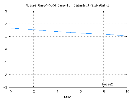
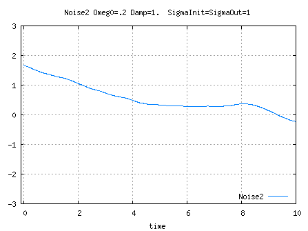
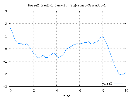
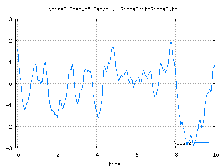
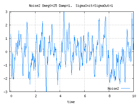
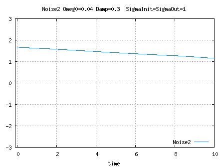
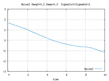
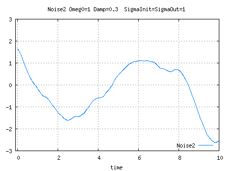
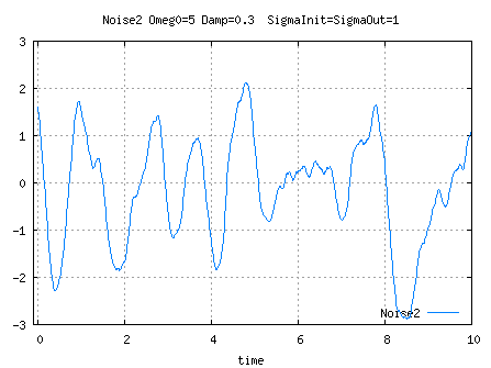
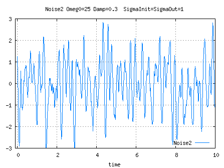
See Parameters computation for K₁, K₀ and A computations.

NF2Noise
//----------------
const float K_StdDevOut=...;
float g_Output2, g_Output, StdDev_WOS, StdDevInit;
//at init time ( I am not 100% sure of the theoretical soundness of g_Output initialization)
void initcoloredNoise2()
{
//to get constant statistical characteristics right from the start
StdDevInit= K_StdDevOut;
//

StdDev_WOS= K_StdDevOut* sqrt(A*(1- K₀)*(1+K₀-K₁)/(1+ K₀));

g_Output2= StdDevInit* RVgauss01();
g_Output= StdDevInit* RVgauss01();
float corr= -K₁/(1+K₀);
g_Output= corr*g_Output2+sqrt(1-corr*corr)*g_Output;
}
//--------------------
float coloredNoise2()
{
float TmpPrevOutput= g_Output;
g_Output= -K₁* TmpPrevOutput- K₀* g_Output2+ StdDev_WOS* RVgauss01();
g_Output2= TmpPrevOutput;
return g_Output;
}

gaussian white noise generator

RVUniform01() returns a random variable with constant probability density=1 on [0,1].

/* RVgauss01() returns a gaussian purely random variable, with mean=0 and standard deviation= 1. Each call to RVgauss01() will return a value uncorrelated with any previous one.*/
double RVgauss01() ( void)
{
static int bSwitch_s= 1;
static double G2_s;
bSwitch^= 1;
if( bSwitch) return G2_s;
double v1, v2, w, y;
do
{
v1= 2.0* RVUniform01()- 1.0;
v2= 2.0* RVUniform01()- 1.0;
w= v1 * v1 + v2 * v2;
} while( w> 1);
y= sqrt( -2.0* log(w)/ w);
G2_s= y* v2;// is independent from y *v1
return y* v1;
}

RVapproxGauss01() is an "approximation" of RVgauss01(), which is probably good enough for use in games.The higher the N, the closer to a white noise probability density.
N=1 returns the uniform probability density on [-0.5, 0.5], N=2 returns a triangle probability density, N=3 a piece-wise parabolic probability density,...
N= 5 is a minimum to have a decent approximation, and N=12 allows code simplification.
Note: as opposed to RVgauss01(), fabs(RVapproxGauss01()) can never be greater than sqrt(3*N).

const int N=...;
const float K_nr= (float)sqrt(12.0f/ N);
float RVapproxGauss01()
{
float x= 0;
for( int i= 0; i< N; i++) x+= RVUniform01()-0.5f;
return x* K_nr;
}