
Equations:
dv/dt= - k1*v+ k0*( u- x)
dx/dt= v
Parameter: k1, k0.
Tuning parameters;{ ω0, ζ } or { ωR, ζ } or { Settling Time, ζ }
Instead of fiddling with k1 and k0, tuning parameters that are
more distinctly related to the wanted behavior of the dynsyst are proposed.
The core tuning parameters are the natural ( un-damped) frequency ( in radian/sec, not in Hertz) ω0 (read omega zero) and
relative damping coefficient ζ (read zeta)
To put it simply:
-for a given ζ, ω0 sets the responsivenes of the dynsyst, ie how
fast its output reaches the input ; "responsiveness" increases with ω0.
-for a given ω0 , ζ sets the damping of the dynsyst( 0< ζ );
damping increases with ζ.
.If ζ< 0, the filter is unstable ( diverging).
.If ζ= 0, the filter produces steady oscillations.
.If 0< ζ≤ 1, the filter produces more or less damped oscillations
( though they are hard to see for ζ> 0.7).
.If ζ≥ 1 ,no oscillation occur; The filter is "over-damped": it is equal to two first order filters placed in a row ( the output
of the first being the input of the second).
The parameters k_1 and k_2 of these first order filters are such as:
ω0= sqrt(k_1*k_2) and ζ= 0.5*(k_1 +k_2)/sqrt(k_1*k_2).
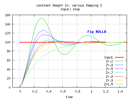
Usual values for ζ are between 0.5 and 0.7 [see Fig N2LL0].
Actually, ζ has also an influence on responsiveness.
I consider a better set of tuning parameters for damped-oscillations
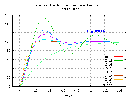
dynsysts ( ie with 0< ζ≤ 1) to be { ωR, ζ } with ω0= ωR/sqrt(1-ζ2) because
ωR is the actual frequency of the oscillations [see Fig N2LLR].
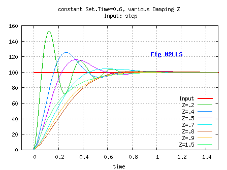
Another convenient set of parameters is { Settling Time, ζ } .
The Settling Time ST is the time after which abs( u-x) stays under Delta=5% of
input when input is a step [see Fig N2LLS].
Due to oscillations for ζ< 1, exact computation of Settling Time ST is complex,
but one can use the following very rough approximation, with Delta=0.05,
for ζ<=0.707 , ω0= -log(Delta)/(ζ*ST).
for ζ>0.707 , ω0= -2*log(Delta)*ζ/ST.
I personally use my function "calcOmeg0FromSetTime()" hereunder,
which gives a better approximation.
For exact computation, see Helper function(s).
float calcOmeg0FromSetTime( float SettlingTimeS_i, float DampCoeff_i)
{
if( DampCoeff_i< .8)
return 3.0f/ (SettlingTimeS_i* DampCoeff_i);
else if( DampCoeff_i< 1.937f)
{
float a= 4.7* exp(1.43940364*log(DampCoeff_i));
return a/ SettlingTimeS_i;
}
else
return 6.0f* DampCoeff_i/ SettlingTimeS_i;
}
With the idea to keep the simple ( I think) tuning parameters setting
process of the continuous dynsyst and to have a numerical dynsyst
behaving like its continuous counterpart, I introduce K1 and K0 defined as
.K1= -2* exp( - T*ω0*ζ) cos ( T* ω0* sqrt(1-ζ2))
and K0= exp( - 2 * T * ω0* x) for damped oscillations dynsysts,
.K1= -( exp(-T*ω1)+ exp(-T*ω2))
and K0= exp(-T*ω1)* exp(-T*ω2) for over-damped dynsysts
having two time constants τ1= 1/ω1
and τ2=1/ω2.
To reduce clutter, I use parameters A=1+K0+K1, B=2+K1 and C= B-A=1- K0
Besides, instead of using variables "finite difference" D= Xn- Xn-1 as usual, I use
whenever possible the rate of increase of output ( pseuso-speed) as V= (Xn- Xn-1)/T
and rate of increase of pseudo-speed (pseudo-acceleration)=(Vn- Vn-1)/T.
This puts forward variables that have a practical meaning to me,
helping when I want to introduce non-linearities (eg: bounds)
and solve the synchronisation/initialisation issues whenever I want to switch between dynsysts.
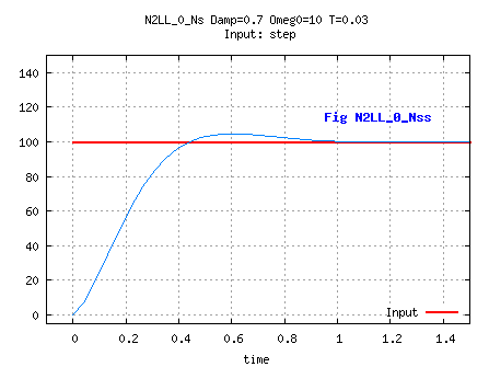
For damped-oscillations dynsysts, sampling imposes the constraint: ω0< π/T; degeneracy actually occurs below
this bound, but the worst does not show until it is crossed.
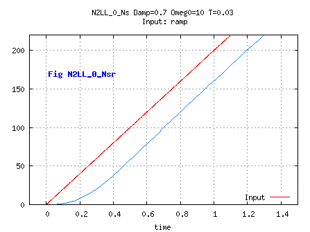
Procedure:
Vn= Vn-1- C* Vn-1+ (A/T)*(Un- Xn-1)
Xn= Xn-1+ T* Vn ie integrating on Vn instead of Vn-1
Parameters : A=(1+K0+K1), C= 1+ K0.
N2LL_1Ns is actually just one step ahead of N1LL0_Ns: with input= Un-1 instead of Un and C= B-A, the behaviour is the same as N1LL0_Ns, at the cost of memorizing U for one step.
By setting A=C=1 one can get a "no-effect" filter.
A convenient feature is that A=1+K1+K0 can be computed for a given ζ
when C= 1-K0 is fixed ( K1 can be expressed as a function of K0 and ζ
see 2nd order stationary linear system).
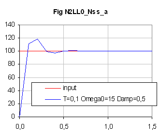
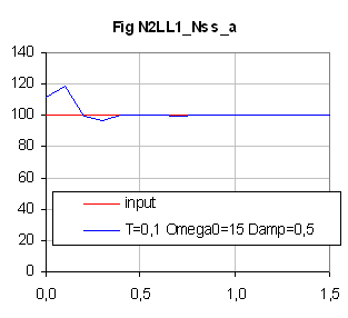
A drawback is that N2LL_1Ns does not behave like expected ( low-pass) for ω0 too close to
π/T, whereas N1LL0_Ns still does its best[ see Fig N1LL0_Nss_a & N1LL1_Nss_a].
Given an ideal acceleration IdealAcc, the most obvious implementation is
AccTmp= minmax( IdealAcc, -ACCBOUND, ACCBOUND);
SpeedTmp= Vn-1+ T * AccTmp;
Vn=minmax( SpeedTmp, -SPEEDBOUND, SPEEDBOUND);
Xn= Xn-1+ T* Vn;
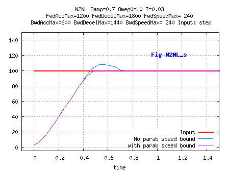
A problem arises if SPEEDBOUND is variable and decreases:
The bound on speed may generate a decrease from Vn-1 to Vn which would implicitely
generate an ( negative) acceleration outside the required acceleration bounds.
The solution is to bound an intermediate speed input and not the ouput speed:
IdealSpeedTmp= Vn-1+T* IdealAcc;
SpeedTmp= minmax( IdealSpeedTmp, -SPEEDBOUND, SPEEDBOUND);
IdealAccTmp= (SpeedTmp- Vn-1)/T;
AccTmp= minmax( IdealAccTmp, -ACCBOUND, ACCBOUND);
Vn= Vn-1+ T* AccTmp;
Xn= Xn-1+ T* Vn;
Besides, the second solution allows for the addition of a perturbation
- at AccTmp level- the effect of which will not be bounded.
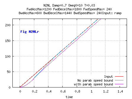
//code needs optimization!
float boundRateNAccAsym( float CurrTimeStep_i, float XInput_i)
{
/*
ForwardAccMax, ForwardDecelMax, BackwardAccMax ,BackwardDecelMax: all >=0
ForwardSpeedBound >0;
BackwardSpeedBound <0;
*/
const K_Epsilonf= .00001f;
float Delta_a;
float Rate_a;
float Acc_a;
float SpeedSgn_a;
Label_1:;
Delta_a= XInput_i- x;
SpeedSgn_a= Rate> 0? 1: (Rate< 0? -1:(Delta_a< 0? -1: 1));
Rate_a= Delta_a/ CurrTimeStep_i;
float RatePar_a;
float DecelMax_a;
//uncomment the following for alternative behaviour
//#define IMPL_PARABSPEEDBOUND
#ifdef IMPL_PARABSPEEDBOUND
//compute max speed to avoid overshoots and bound Rate_a accordingly
if( SpeedSgn_a> 0) DecelMax_a= ForwardDecelMax;
else DecelMax_a= BackwardDecelMax;
RatePar_a= -0.5* DecelMax_a* CurrTimeStep_i+ sqrt( 2* DecelMax_a*fabs(Delta_a));
if( RatePar_a> 0)
{
if( Rate_a> RatePar_a) Rate_a= RatePar_a;
else if( Rate_a< -RatePar_a) Rate_a= -RatePar_a;
}
#endif
//standard speed bound
if( Rate_a> ForwardSpeedBound) Rate_a= ForwardSpeedBound;
else if( Rate_a< BackwardSpeedBound) Rate_a= BackwardSpeedBound;
// acceleration bound
Acc_a= (Rate_a- Rate)/ CurrTimeStep_i;
if( SpeedSgn_a< 0)
{
if( Acc_a> BackwardDecelMax) Acc_a= BackwardDecelMax;
else if( Acc_a< -BackwardAccMax) Acc_a= -BackwardAccMax;
}
else
{
if( Acc_a> ForwardAccMax) Acc_a= ForwardAccMax;
else if( Acc_a< -ForwardDecelMax) Acc_a= -ForwardDecelMax;
}
Rate_a= Rate+ CurrTimeStep_i* Acc_a;
// handle speed sign change with a lerp based on time
if( (Rate_a> K_Epsilonf && Rate< -K_Epsilonf)||( (Rate_a< -K_Epsilonf && Rate> K_Epsilonf)))
{
CurrTimeStep_i= CurrTimeStep_i- Rate/ Acc_a;
Rate= 0;
goto Label_1;/*yes, I know...so I'll take the usual easy way out: re-writing the code without goto is left as an exercise to the reader.*/
}
//update
Rate= Rate_a;
x= x+ CurrTimeStep_i* Rate_a;
return x;
}
Procedure:
Prediction: Ve= Vn-1; Xe= Xn-1+ T*Vn-1.
Correction: Vn= Ve+ (A/T)* ( Un- Xe); Xn= Xe+ C* ( Un- Xe).
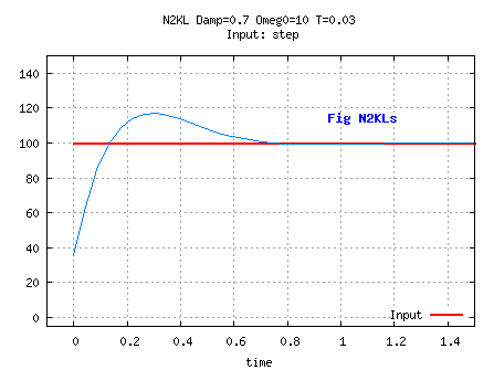
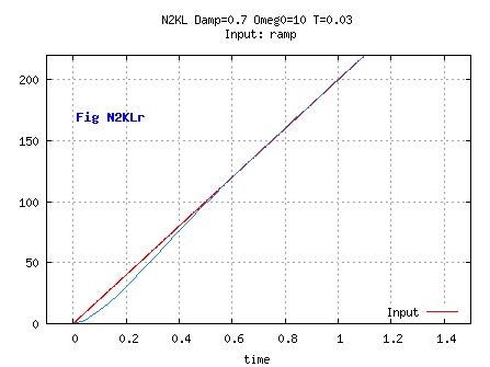
This is a tweak of N2KL no longer used as an estimator,
by changing variables so as to show ouput rate
and acceleration to be able to bound them.
I also introduce a state, in order to be able to reset the dynsyst
when the information that the input variation (Un- Un-1)/T should not be interpreted as a speed
is available, corresponding to State=0 ( eg: changing target for a dynsyst applied to a view angle).
If this information is available, the dynsyst should be initialized with State= 0.
If not, the dynsyst should be set with State= 1 forever;
it may then show a noticeable overshoot on a big step input.
The next enhancement would be to introduce asymetry as in boundRateNAccAsym,
but with ForwardAccMax= BackwardAccMax,
ForwardDecelMax= BackwardDecelMax and BackwardSpeedBound=-ForwardSpeedBound.
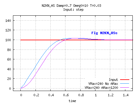
Depending on the values of A, C, ACCBOUND and SPEEDBOUND,
the bound on acceleration may generates noticeable overshoots,
especially with dynsysts with high ω0.
The bound on acceleration must be understood as a bound
on the rate of increase/decrease of the speed variable.
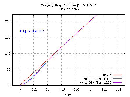
//A= 1+ K0+ K1;
//C= 1-K0;
//float x, v, PrevInput, State;// globals
//at init time: v=..., Input=x=...,State= 0;
float N2KN_AS( float CurrTimeStep_i, float CurrentInput_i)
{
float Delta_a= PrevInput- x;
float Vc_a;
if( State!= 1)
{
Input= CurrentInput_i;
State= 1;
}
if( CurrentInput_i== PrevInput)
{
Delta_a= wrapHalfPrd(Delta_a) ;
Vc_a= (A/C)* Delta_a/ CurrTimeStep_i;
}
else
{
float DeltaNew_a= CurrentInput_i- x;
DeltaNew_a= wrapHalfPrd(DeltaNew_a) ;
Delta_a= wrapHalfPrd(Delta_a) ;
Vc_a= ( ((A/C)-1)* Delta_a+ DeltaNew_a)/ CurrTimeStep_i;
//or? TO DO test on angles
//float DeltaCbn_a= wrapHalfPrd((A/C)-1)* Delta_a+ DeltaNew_a);
//Vc_a= DeltaCbn_a/ CurrTimeStep_i;
}
float V1_a= v+ C* ( Vc_a- v);
V1_a= minmax( V1_a, -SPEEDBOUND, SPEEDBOUND);
float Acc_a= (V1_a- v)/ CurrTimeStep_i;
Acc_a= minmax( Acc_a, -ACCBOUND, ACCBOUND);
v= v+ CurrTimeStep_i* Acc_a;
PrevInput= CurrentInput_i;
x= x+ CurrTimeStep_i* v;
x= wrapPrd(x) ;
return x;
}
int calcF2CoreParams( float T_i, float Omega0_i, float DampCoeff_i
, float & k1_o, float & k0_o)
{
// this function computes the core parameters for a 2nd order numerical filter
// T_i: expected Timestep
DBGASSERT( 0< DampCoeff_i);
float K_a= exp( - T_i* Omega0_i* DampCoeff_i);
k0_o= K_a* K_a;
k1_o= -2* K_a;
float OmegaR_a= Omega0_i* sqrt(fabs(1.0f- DampCoeff_i*DampCoeff_i));
if( DampCoeff_i<= 1)
{
//DBGASSERT( Omega0_a< (M_PI/ T_i));
k1_o*= cos( T_i* OmegaR_a);
}
else
{
k1_o*= cosh( T_i* OmegaR_a);
}
return 0;
}
static float calcSTOmgInf1( float DampCoeff_a, float ProportionalError_a);
static float calcSTOmgSup1( float DampCoeff_a, float ProportionalError_a);
//--------------------------------------------------------------
float calcSTOmeg0FromSetTime( float DampCoeff_i, float ProportionalError_i)
{
/* this function return the exact value of SettlingTime*Omeg0 for a continuous 2nd order low-pass filter where SettlingTime is the time after
which abs(input-ouput)< (ProportionalError_i* input) when input is a step.*/
if( DampCoeff_i> 1.0f)
return calcSTOmgSTSup1( DampCoeff_i, ProportionalError_i);
else if( DampCoeff_i< 1.0f)
return calcSTOmgSTInf1( DampCoeff_i, ProportionalError_i);
else //DampCoeff_i== 1.0f
return 4.744f;
}
//------------------------------------------------
float calcSTOmgInf1( float damp_a, float prop_a)
{
float x0, x;
float y0, y;
float s= sqrt( 1.f-damp_a*damp_a);
int k=0;
while( exp(-k*M_PI*damp_a/s)> prop_a) { ++k;}
x0= (k-1)*M_PI/s;
y0= exp(-x0*damp_a)*((k&1)?1:-1);
if( y0< 0) prop_a=-prop_a;
y0= y0- prop_a;
x= (k*M_PI-atan(s/damp_a))/s;
y=- prop_a;
while( fabs(y)>0.00001)
{
x=x0-y0*(x-x0)/(y-y0);
y= exp(-x*damp_a)*( cos(x*s)+sin(x*s)*damp_a/s)- prop_a;
float xPrev= x;
}
return x;
}
//------------------------------------------------
float calcSTOmgSup1( float damp_a, float prop_a)
{
float x0, x;
float y0, y;
float s= sqrt( damp_a*damp_a-1.f);
float a= prop_a*2*s;
x= -2*log(prop_a)*damp_a;
y= (damp_a+s)*exp(-x*(damp_a-s))-(damp_a-s)*exp(-x*(damp_a+s))-a;
x0= x;
y0= y;
x= 3/(2*damp_a);
while( fabs(y)>.00001)
{
y= (damp_a+s)*exp(-x*(damp_a-s))-(damp_a-s)*exp(-x*(damp_a+s))-a;
float xPrev= x;
x=x0-y0*(x-x0)/(y-y0);
x0=xPrev;
y0=y;
}
return x0;
}