
Equation:
dx/dt= k(u- x) where u is the input, x is the ouput and dx/dt is the first derivative of x.
Parameter: k.
Tuning parameter: { k> 0 } or Time Constant{ τ= 1/k} or Settling Time {ST= 3*τ= 3/k }.
The Settling Time is the time after which abs( u-x) stays under 5% of
input when u is a step.
if k is negative, the dynsyst is unstable ( divergent): x grows exponentially.
if k is positive, it is stable ( convergent) : x moves towards u.
The greater k is, the faster x reacts to a change in u.
Behavior
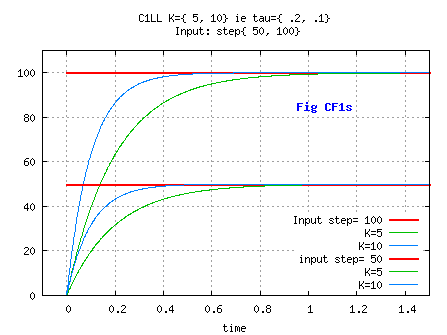
On a unit step input ( u(t< 0)=0, u(t≥ 0)= U0 with U0 constant) [see Fig C1Fs]
As a function of time: x= ( 1- exp(-k*t) )* U0 for t<0.
x reaches approx. 63% of U0 at t= 1/k= τ.
x reaches approx. 95% of U0 at t= 3/k= 3*τ= Settling Time by definition.
x reaches approx. 99% of U0 at t= 4.6/k= 4.6*τ.
x reaches approx. 99.9% of U0 at t= 7/k= 7*τ.
dx/dt at t=0 ( ie x slope ) is equal to U0*k= U0/τ.
When t is big enough, exp(-k*t)≅ 0 then x≅ U0.
If x0 is not null, then x= x0+ ( 1- exp(-k*t))* (U0- x0).
Its integral is y= ∫ x= y0+ t* U0- ( U0- x0)* (1- exp(-k*t))/ k, or y= y0+ t* U0- ( x- x0)/ k.
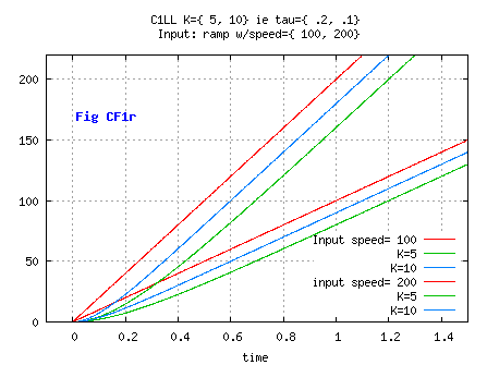
On a ramp input ( u(t< 0)=0, u(t≥ 0)= USpeed*t with USpeed constant) [see Fig C1Fr]
Then x= USpeed*( t- (1- exp(-k*t))/k ) for t≥ 0.
When t is big enough: x ≈ USpeed*( t- 1/k) ie x ≈ u- USpeed/k.
We face here an unavoidable drawback of the first order low-pass filter:
on a ramp input, its output x will always "lag" behind the input u, by a value USpeed/k.
More generally, when the input signal varies with time, there is no way for the ouput
to get close to the input.
As the error is known, one can think to compensate for it by adding a
USpeed/k term to u ( or a portion of it).
This does not work as the filter looses its low-pass behaviour.
Another way would be to introduce another low-pass filter fed in by USpeed,
providing a smoothed speed used in the compensating term.
This would lead to using two first order filters and effectively,
the only solution for inputs varying as a ramp, ie u proportional to t, is to
use a "special" second order dynsyst.
This is addressed in a cleaner way in the 2nd order dynsysts chapter.
More generally, for inputs u proportional to tn a "special"
(n+1) order dynsyst is required.
Procedure:
The standard format is: Xn= K* Xn-1 + (1- K) Un-1,
but I prefer: Xn= Xn-1 + A* ( Un-1 - Xn-1 ), where A= 1-K.
Parameter: 0 ≤ A ≤ 1
Tuning parameter:
{ k>0 } then A= 1- K= 1-exp(-k*T), or Time Constant { τ>0 } then A= 1-exp(-T/τ)
or Settling Time { ST> 0}, then A= 1-exp(-3*T/ST).
Behavior:
Assuming U= X= 0 for n< 0...
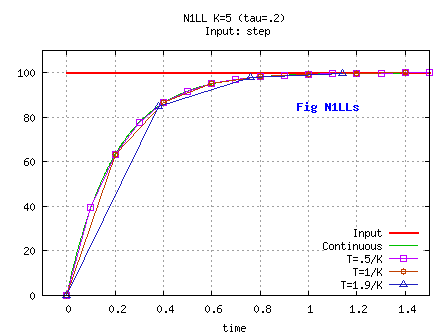
On a step input ( U(n< 0)=0, U(n≥ 0)= U0 with U0 constant≠ 0) [see Fig N1LLs]
At t=n=0: X= 0;
At n=1, t=T: X= A* U0;
Analytical expression, assuming a non null initial condition X0: Xn= (1- Kn)*U0+ Kn X0.
Assuming X is the input of an integrator such as IXn= IXn-1+ T* Xn-1, then
IXn= IX0+ T*( n*U0+ ( X0- U0)*( 1- Kn)/( 1-K))
If X is a speed, and IX a position, assuming X0 > 0 and U0=0 ( ie a stop order), the distance run until full stop is:
StopDist= T*X0/(1-K)= T*X0/A ( idem if IXn= IXn-1+ T* Xn).
Using this result the other way round, for a mobile the speed dynamics of which obey the X equation, the last formula gives the distance to its final destination at which its speed must be set to zero in order to stop right on target ( prediction).
On a step input, N1LL matches perfectly the continuous filter values, even with high values of timestep.
Procedure:
Xn= Xn-1 + A * ( Un - Xn-1 ), ie same as N1LL, except for the input which is here the current step value
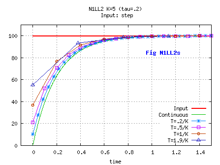
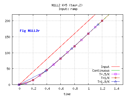
Behavior: N1LL_Ns is one step ahead of N1LL.
Assuming U= X= 0 for n< 0...
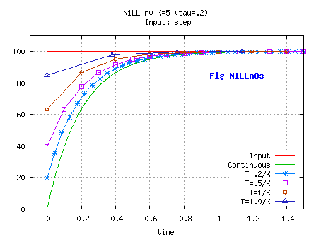
On a step input ( U(n< 0)=0, U(n≥ 0)= U0 with U0 constant≠ 0) [see Fig N1LLn0s]
At t=n=0: X= A*U0 , ie the dynsysts reacts right away at t=n= 0.
Analytical expression, assuming a non null initial condition X0: Xn= (1- Kn+1) * U0+ Kn X0;
Assuming X is the input of an integrator such as IXn= IXn-1+ T* Xn-1 , then
IXn= IX0+ T*( n*U0+ (X0- U0)*K *( 1- Kn)/( 1-K)).
If X is a speed, and IX a position, assuming X0 > 0 and U0=0 ( ie a stop order), the distance run until full stop is :
StopDist= T*X0* K/(1-K)= T*X0*(1-A)/A ( idem if IXn= IXn-1+ T* Xn).
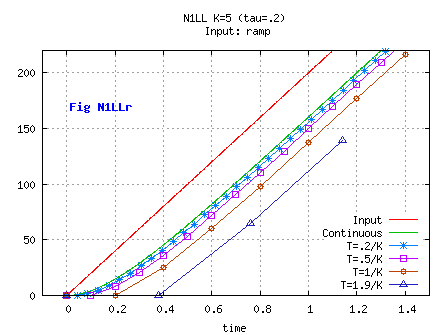
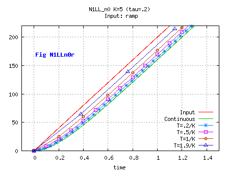
On a ramp input ( U(n< 0)=0, U(n≥ 0)= USpeed*n*T with USpeed constant) [see Fig N1LLn0r]
At t=n=0: X= 0.
In steady state, Un- Xn= USpeed*T(1-A)/A; the error is not equal to zero.
Notes :
1.if A= 0 ( zero reaction time, ie k= infinite) then for N1LL_Ns: Xn = Un ie N1LL_Ns is "transparent" as one could expect,
whereas for N1LL: Xn = Un-1 ie N1LL introduces a one Timestep pure delay.
This tends to make N1LL_Ns a better choice.
The drawback is that, for a given k, N1LL_Ns smoothes less when the Timestep is increasing, wich is counter intuitive.
2.N1LL_Ns can be used as a first order estimator:
U is then the unknown modelled as a constant, X is its estimate,
which must initialized to the best guess for U.
3.N1LL and N1LL_Ns have the same source code, as the input is
an argument of the calling function implementing them.

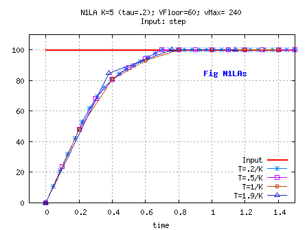
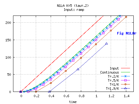
on a unit step input
For large initial values of U-X and proper setting of
SPEEDFLOOR and SPEEDBOUND, the first portion of X curve is at constant rate= SPEEDBOUND,
the second portion is as a linear filter , and the last portion
is at constant speed= SPEEDFLOOR until X reaches U.
float N1LA_angle( float CurrTimeStep_i, float Output_i/*previous output*/, float Input_i)
{
float Delta_a= Input_i- Output_i;
Delta_a= wrapHalfPrd( Delta_a );
float Rate_a= Delta_a/ CurrTimeStep_i;
float RateRBnd_a= minmax( Rate_a, -SPEEDFLOOR, SPEEDFLOOR);
float RateLin_a= A* Rate_a;
if( Rate_a>= 0) Rate_a= RateRBnd_a> RateLin_a? RateRBnd_a: RateLin_a;
else Rate_a= RateRBnd_a< RateLin_a? RateRBnd_a: RateLin_a;
Rate_a= minmax( Rate_a, -SPEEDBOUND, SPEEDBOUND);
Output_i= Output_i+ CurrTimeStep_i* Rate_a;
Output_i= wrapPrd(Output_i) ;
return Output_i;//updated output
}

The purpose is the same as for N1LA, but implementation and behaviour are different
I compute the speed as for a rate bounder,
split it with a first order filter parameter A
, bound the (1-A)Speed term to SPEEDFLOOR, and finally re-combine ( add) the two terms.
Behavior:
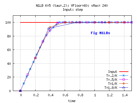
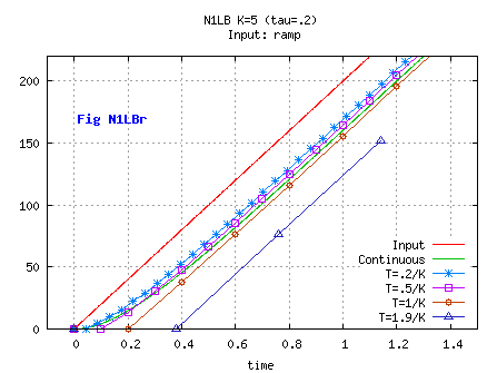
on a unit step input
For large initial values of U-X and proper setting of
SPEEDFLOOR and SPEEDBOUND, the first portion of X curve will be at constant rate= SPEEDBOUND,
and the second and last portion will be as a linear dynsyst,
X reaching for U at rate = SPEEDFLOOR.
float N1LB_Angles( float CurrTimeStep_i, float Output_i/*previous output*/, float Input_i)
{
float Delta_a= Input_i- Output_i;
Delta_a= wrapHalfPrd( Delta_a);
float Rate_a= Delta_a/ CurrTimeStep_i;
Rate_a= minmax( (1-A)* Rate_a, -SPEEDFLOOR, SPEEDFLOOR)+ A* Rate_a;
Rate_a= minmax( Rate_a, -SPEEDBOUND, SPEEDBOUND);
Output_i= Output_i+ Rate_a * CurrTimeStep_i;
Output_i= wrapPrd(Output_i) ;
return Output_i;
}