My approach to numerical dynsysts design is different than the one game
programmers can usually read about, and this explains why and in what way,
with several examples. This can be helpful for those who want to create their own dynsyst/filter and those whose face an unexpected behaviour of their code.
The widespread approach, referred to as "A" in the following, is
- to select a continuous dynsyst known as behaving as required( eg: the good ole' spring and damper system),
- then to set the dynamic characteristics ( stability/damping and responsiveness) by tuning the parameters of the
equations of the continuous model,
- and last to select an integration scheme to get a set of numerical equations.
This approach has some pitfalls:
- it can lead to unnecessary complicated numerical equations ( resulting
from the integration scheme), eventhough a 100% faithfull simulation might not be an objective,
- sampling ( and possibly the integration scheme)
generates its own stability problems which cannot
be addressed based on the continuous system analysis.
As a consequence, the numerical dynsyst may show for certain
values of parameters and/or for high values of the timestep the dreaded "weird" behavior,
while not knowing why and how to prevent that.
The main issue is the underlying assumption in "A" process that stability and responsiveness characteristics of the continuous system will be carried over to the numerical system.
This is unfortunately not true, theory tells that stability analysis is different between the two type of systems.
This is why my approach, referred to as "B" in the following, departs from the usual approach
by applying their own appropriate rules to the numerical dynsysts;
I also sometimes allow myself to forget about the 100% faithfull simulation of a continuous system.
Speed=( Input? - Outputn-1)/T;
if (Speed> SPEEDBOUND) v= SPEEDBOUND;
else if( Speed< -SPEEDBOUND) v= -SPEEDBOUND;
Outputn= Outputn-1+ T* Speed;
Speed=( Inputn-1 - Outputn-1)/T;
Assuming input(t< 0)=output(t< 0)=0, then, at t= 0 (corresponding to n=0) on a large enough step input, Output0= Inputn-1= 0.
-"B" standpoint : considering that bounding the speed of Input is really
the only purpose of the design, I do not refer to the continuous case at all,
and I can write directly the simplest equation that fits the need, with Input argument= current value of Input.
Speed=( Inputn - Outputn-1)/T;
The behavior is different:
Approach "B" does not introduce an one time-step lag (pure delay).
This lag can create problems when several numerical dynsysts/filters are placed in a row ( one step pure
delay is introduced for each of the dynsyst).
Moreover, I expect the filter to have no effect whenever the absolute value
of the input speed stays under the max speed. "B" fulfills this requirement, but not "A".
On the other end, for "B", the greater the timestep T, the closer the output to the input for a step input
, which is counter-intuitive when expecting a smoothing behavior.
As a conclusion, when the choice is open, I always use "B".
More generally, if I really need a behavior such as "A" with
several dynsysts in a row ( one and only one step delay), I use "B" for all of them except one, or simply add the lag to the first input or to the last output.
A case where Input= Inputn-1 is preferable is when using complementary filters ( 2 filters are complementary when "fed in" with the same input, the sum of their output is equal to the input for all t or n; the highpass filter one should use Inputn whereas its companion lowpass filter should use Inputn-1).
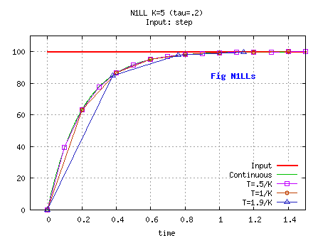
The equation of the continuous 1st order low-pass filter is
dx/dt= k( u-x), u being the input, x the output and k the parameter.
A1.1.Deriving the numerical design using a simple integration scheme
Vn= k*(Un- Xn) and Xn= Xn-1+ T*Vn-1.
Then Xn= Xn-1+ k*T*(Un-1- Xn-1).
A1.2.Deriving the numerical design using an implicit integration scheme
Vn= k*(Un- Xn) and Xn= Xn-1+ T*Vn,
then Xn= Xn-1+ (1/(1+k*T))*(Un- Xn-1)
A1.3.Deriving the numerical design assuming constant acceleration
Vn= k*(Un- Xn) and Xn= Xn-1+ 0.5*T*(Vn+Vn-1).
Then Xn= Xn-1+ (k*T/(1+0.5*k*T))*( 0.5*(Un+Un-1)- Xn-1)
A2. Selecting a particular input, finding x as a function of time,
and deriving a numerical system by allowing any input.
With a step as input,
dx/dt= k( u- K_UO), with u= K_UO being the constant step value for t≥ 0;
then for t≥ 0:
x= x0* exp( -k*t)+ ( 1- exp( -k*t))* K_U0
or x= x0+ ( 1- exp(-k*t))* (K_UO- x0)
Endly, releasing the constraint that the input be a step, and considering x values
between 2 steps with T= t:
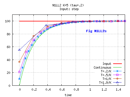
Xn= Xn-1+ (1- exp(-k*T))*(Un-1- Xn-1)
K_U0 is replaced by Un-1 to insure X0= x0= 0.
Whatever T, even if variable, on a step input the output will be equal to the continuous one.
because the continuous equation has been solved for such an input.
This does not holds true for other inputs.
Stability analysis ( not detailed here) results in the following constraints:
0< 1-A < 1, ie 0< A< 1.
Neither "A1.1" nor "A1.3" solutions guarantee that.
"A1.2" and "A2" solutions are OK, though "A1.2" will obviously not provide
an output similar to the one of the continuous system.
One can set parameter A directly, but my choice is to have the numerical system getting
the same stability characteristics as the continuous one
( the roots of the characteristic equation of the numerical dynsyst
are function of those of its continuous counterpart).
Here, this fully defines A ( and K= 1- A) as A= (1- exp(-k T)).
"A2" solution, though resulting from a process not involving stability criteria,
fulfills the stability requirement and even gets the same formula for A,
but this does not always work.
I prefer then to use stability analysis, because
-I use a robust process consistent with my main goal, which is to insure stability and
not to model a continuous system,
-getting the analytical solution of more complex continuous
equations quickly becomes a nightmare,
-I can use its criteria for non linear systems.


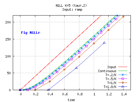
The input is then u= u0+ K_Vc* t, with K_Vc a constant speed.
dx/dt= k( u- x)
Then for t≥ 0:
x= (u0-x0)* exp(-kt)- u0+ K_Vc* ( t- (1- exp(-kt))/ k),
then, as K_Vc= (u- u0)/ t:
x= x0*exp(-kt) + u0*(1- exp(-kt))+ (u- u0)*(1- (1- exp(-kt))/(kt))
or x= x0+ (1- exp(-kt))*(u0- x0)+ (u- u0)*(1- (1- exp(-kt))/(kt))
Endly, releasing the constraint that the input be a ramp, considering x values
between 2 steps with T= t and introducing A= 1-exp(-kT):
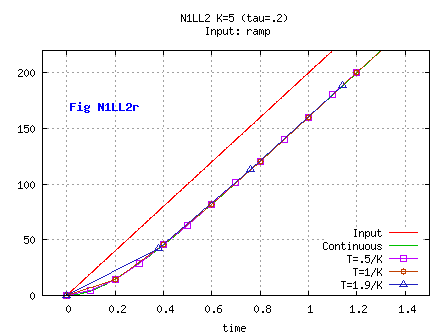
Xn= Xn-1+ A*(Un-1- Xn-1)+ (Un- Un-1)*(1-(1- A)/(kT))
A correcting term appear compared to the previous system.
Introducing b defined as b= 1/A- 1/(kT),
the process can be split into two steps:
UTemp= Un-1+ b*(Un- Un-1), ie a combination of the inputs ( actually a non recursive filter),
and Xn= Xn-1+ A*(UTemp- Xn-1), which is the equation seen in the preceding paragraph.
Whatever T, even if variable, and on a ramp input, the output will be equal to the output of continuous filter.
This does not holds true for other inputs, including a step input.
Note that the stability criterion is the same as before ( 0< A <1), and the behavior has been changed by modifying the input.


This study elaborates on the preceding one, with a filter which is non-linear.
My specification is that the output should decelerate at a max deceleration a
when moving from its current value towards the input, when the input is a step.
Here, I use "A2" process just to get a set of equations, and end with stability analysis.
From the specs, x is a parabola that must pass through the previous output x0=x(t=0),
and through the constant input U= K_UO with a null speed;
after having reached the input, the parabola should obviously not apply anymore.
The equations should give the remaining unknown, ie the current speed and
finally the set of equations.
Obviously, the speed should have the same sign as K_UO-x0,
and the acceleration should have the opposite sign.
for any point between x(t=0) and K_UO:
x= x0+ v0* t- 0.5* Sgn* a* t2
with a> 0 being the deceleration, Sgn the sign of ( K_UO-x0)
, x0 and v0 being the value and speed at t= 0
K_UO must be the apex reached at tf where vf= v(tf)= 0,
tf= t0+ abs(v0)/a.
Hence, v0 must be such as K_U0= x0+ 0.5*Sgn*v02/ a
ie v0= Sgn* sqrt( 2*a*abs(K_U0-x0)), which gives
x= x0+ Sgn* sqrt( 2*a*abs(K_U0-x0))* t- 0.5*Sgn*a*t2.
With T= t, x0= Xn-1, and replacing the constant K_U0 by any input...
Xn= Xn-1+ T * Rate, with Rate= Sgn*( -0.5*a*T+ sqrt( 2*a*abs(Un- Xn-1))).
We wind up with a non linear 1st order dynsyst.
Translating stability requirement on parameter A from the preceding example
results in the requirement that Rate as above be replaced by (Un- Xn-1)/T
whenever abs(Un- Xn-1)/T ≤ 0.5*a*T.
Actually, instead of using Rate as a command and forcing x to a parabola,
using it as a bound provides more flexibility; the final pseudo-code is then:
Rate= (Un- Xn-1)/T // or any lower value with the same sign implementing possible additional constraints from specs;
if( abs(Rate)> 0.5*a*T)
{
RateParabMaxTmp= ( -0.5* a* T+ sqrt( 2*a*abs(Un- Xn-1)));
if( Rate> 0) Rate= RateParabMaxTmp;
else Rate= -RateParabMaxTmp;
}
Xn= Xn-1+ T * Rate;